Approximate Bayesian Computation (ABC)
What to do when you do not have a likelihood? One of the answers for this question is the Approximate Bayesian Computation (a.k.a. ABC). This bayesian approach can be used to solve several problems in Statistics, e.g. to compare models, regressions, etc.
In summary, the ABC algorithm works as follows:
- Once the model and its parameters \(\theta_i\) are defined, the algorithm samples the parameter space by generating a large enough set of values, following the parameter priors \(P(\theta_i\)).
- The distances between the data and the sampled model, generated in the previous step, are calculated: \(D_i(y_i, y_{model, i}\)).
- The posterior of parameters space is built using a small fraction of the \(\theta_i\) which is defined as \(D_i \le \epsilon\). In general, the threshold value \(\epsilon\) is defined as a function of percentiles.
Note that we do not use any Figure-of-Merit to say that the parameter set \(\theta_i\) is good or bad. The only one metric is the comparison between the sampled model and the observed data.
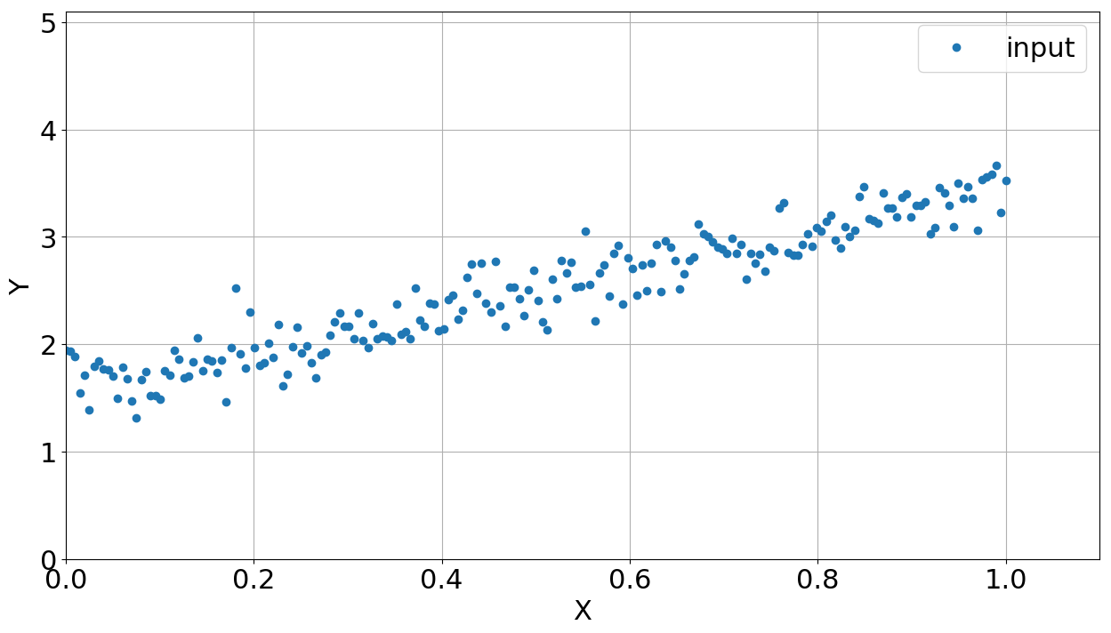
Back to the real world, let's suppose a simple problem to be solved here. You have some data (\(x_i\), \(y_i\)) which clearly demands a linear fitting, i.e., \(y_i = a x_i + b\) (\(a\) and \(b\) correspond to \(\theta_i\)). It is important to say that this data also has some noise. Figure 1 shows the correlation between \(x_i\) and \(y_i\). How to fit a linear equation here? Maybe you can just use the \(\chi^2\) as the Figure-of-Merit and find the best values of \(a\) and \(b\) by exploring the parameter space and comparing the models. But let's suppose you do not know the \(\chi^2\) reduction and you have to fit a linear function on the data. Thus, we start a Python code by loading packages:
              import numpy as np

              import matplotlib.pyplot as plt

              import pymc3 as pm
After that, we might define a function or routine to generate some linear behavior of a mock data, also including some noise into the \(y\) array.
def generate_mock_data(n_points, a0, b0):
"""
Generate some mock data (linear)
"""
x = np.linspace(0., 1., n_points)
epsilon = np.random.normal(0., 0.2, n_points) # gaussian noise
y = (a0 * x + b0) + epsilon
return x, y
Figure 1 shows the data generated by this routine using gaussian noise. The next routine draws the parameter space and calculates the distance between the modelled and observed data.
def
draw_sample(n, a_range, b_range):
"""
Draw n parameters sets of a and b
"""
# Assuming FLAT priors for a and b.
#a_draw = np.random.uniform(a_range[0], a_range[1], n)
#b_draw = np.random.uniform(b_range[0], b_range[1], n)
# Assuming a gaussian prior of a and b.
a_draw = np.random.normal(np.mean(a_range), 0.2, n)
b_draw = np.random.normal(np.mean(b_range), 0.2, n)
# Calculate distances
dist_draw = np.zeros(len(a_draw))
for i in range(len(a_draw)):
y_draw = a_draw[i] * x + b_draw[i]
dist_draw[i] = sum(abs(y_draw - y))
return a_draw, b_draw, dist_draw
where the variables a_range and b_range correspond to the \(a\) and \(b\) ranges to be sampled, respectively. Note that our result is sensitive to the priors functions, being uniform or gaussian functions over the parameter space. Then we start defining some values to generate the mock and to sample the parameter space.
              n_draw = 50000 # sampling number
              a0 = 2. # input slope coefficient
              b0 = 1.5 # input interception coefficient
              a_range = [0.1, 3.] # slope coefficient range
              b_range = [0.1, 3.] # interception coefficient range

              n_points = 200 # input number of points

              threshold = 1.5 # threshold of smallest distances (in percentage)

              n_posterior = 30 # number of posterior models to be plotted

              np.random.seed(123456789) # seed number
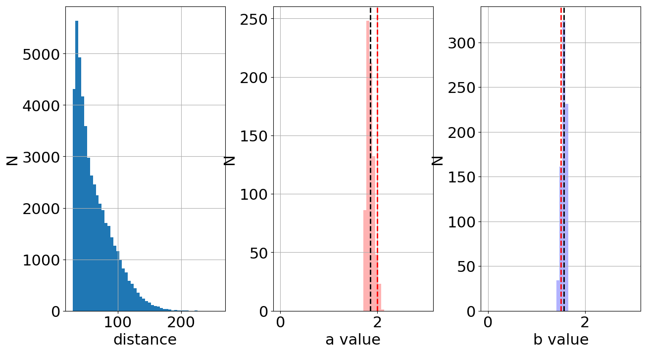
Now we generate the data, run the sampling and calculate the distance for each parameter set \(a\) and \(b\). In total, there are 50000 sets. Figure 2 shows the total distribution of distances (left), the "best" values of \(a\) (center) and the "best" values of \(b\) (right). Note that imposing low values of the variable \(threshold\), it only selects the closest/best models to reproduce the observed data.
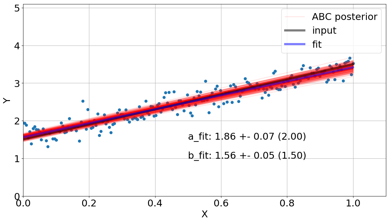
It seems we almost got our goal, right? Wait a minute..let's check the fit done by the algorithm. Figure 3 shows the linear regression and the input data using gaussian priors for \(a\) and \(b\) (check function draw_sample). Note that our model got close (visually) in order to reproduce the data but the output values of \(a\) and \(b\) are not in agreement with the input ones. It is shown in the figure, considering the uncertainties in 1\(\sigma\).
draw_sample including uniform priors and check our new fit.
                  # Assuming FLAT priors for a and b.

                  a_draw = np.random.uniform(a_range[0], a_range[1], n)
                  b_draw = np.random.uniform(b_range[0], b_range[1], n)
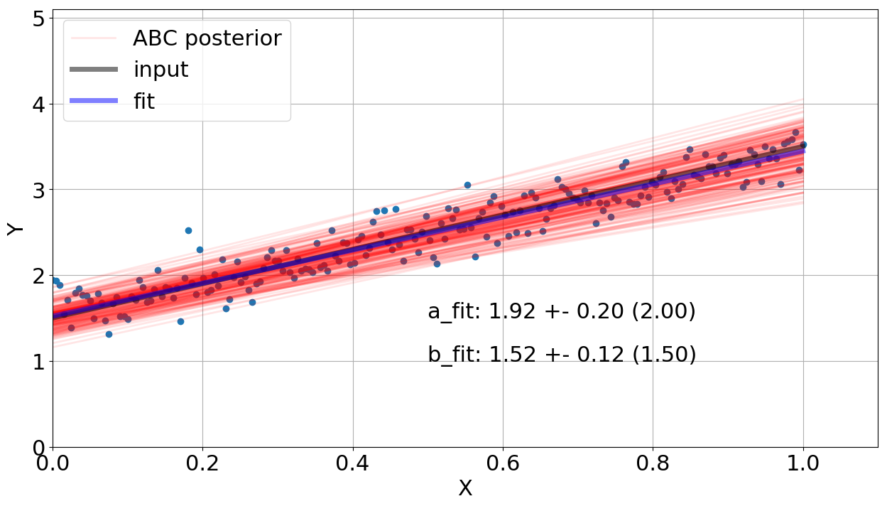
By running the code again, Figure 4 shows our new fitting using now uniform priors for \(a\) and \(b\), covering the parameter ranges defined above. Two things to notice here: 1 - The dispersion of fit values is visually higher, 2 - the fit values got closer to the input values but they include the input parameters in 1 \(\sigma\)).
What is the best prior and threshold value? It is a good question and strongly depends on your problem. For this problem, the gaussian prior did not include the solution in 1 \(\sigma\) but presented lower dispersion. From this point of view, it seems that the gaussian choice did not sample properly the parameter space. Once using the uniform one, our solution is in agreement with the input parameters but the error bars for \(a\) and \(b\) are larger. Out of this scenario, if your likelihood is known and not computationally quite expensive to be calculated, I would not recommend you to use ABC. For instance, some \(\chi^2\) reduction-based method should be employed to fit your model to the data. This algorithm is only suggested when your likelihood is quite complicated or unknown. If you want the code of this post, just check my GitHub repository ABC. If you have any question or comment, just drop me an e-mail.
Some references: