Artificial Neural Networks - Part 2: BackPropagation
def
foward_propagation(X, model):
"""
Foward Propagation
"""
W1, b1, W2, b2 = model['W1'], model['b1'], model['W2'], model['b2']
z1 = X.dot(W1) + b1
a2 = tanh(z1, deriv = False)
z2 = a2.dot(W2) + b2
a3 = softmax(z2)
return a3
being the activation function between the Input and Hidden Layer a tanh(x) and a softmax(x) between the Hidden Layer and the Output Layer. The values of weights and bias arrays are started in a randomic way and at the first iteraction or epoch, the prediction and classification is quite bad.
In this way, our next step is to update the weights and bias arrays after each iteraction (Foward Propagation) in order to get closer to the desired goal. The Back Propagation calculates the difference between the obtained and target values at the output layer and calculates the gradient of weights and bias to update them. The Gradient Descent is employed here and it is based on the derivatives of the loss function \(E\) as a function of the weights and bias, i.e., $$ W_i \leftarrow W_i - \epsilon \frac{\partial E}{\partial W_i} \ \ \ \ \ ;\ \ \ \ \ b_i \leftarrow b_i - \epsilon \frac{\partial E}{\partial b_i}$$ where \(\epsilon\) is known as learning rate.
The loss function can be defined in several ways but here we define it as an error function. Then, $$ E = \frac{1}{2} \sum_i(a_{3,i} - Y_i)^2 $$ where \(Y\) represents the target values of classification or regression and \(a_{3,i}\) is the i-th term of the Output Layer array. According to the equation of Gradient Descent above, our next step is to calculate the derivatives of loss function. Using the Chain Rule, we can write these terms as $$ \frac{\partial E}{\partial W_2} = \underbrace{\frac{\partial E}{\partial a_3}}_{1} \underbrace{\frac{\partial a_3}{\partial z_2}}_{2} \underbrace{\frac{\partial z_2}{\partial W_2}}_{3} $$ and each derivative (1, 2 and 3) can be calculated in a separated way. The first term can calculated as the partial derivative of the sum, $$ \frac{\partial E}{\partial a_3} = \frac{\partial}{\partial a_3} \left(\frac{1}{2}\sum_i(Y_i - a_{i,3})^2 \right) = (a_{i,3} - Y_i)$$ The second term is basically the derivative of the activation term, $$ \frac{\partial a_3}{\partial z_2} = \frac{\partial}{\partial z_2}\left( \sigma_2(z_2)\right) = \sigma_2'(z_2) $$ Note that the derivative of the tanh(x) function is \(1 - tanh(x)^2\), if you want the check the deduction of that, check this link . The last and third term can be written as, $$ \frac{\partial z_2}{\partial W_2} = \frac{\partial}{\partial W_2}\left( \sum a_2 * W_2 + b_2 \right) = a_2 $$ Putting all terms together, the derivative of the error function regards \(W_2\) can be defined as, $$ \frac{\partial E}{\partial W_2} = \underbrace{(a_3 - Y)}_{\delta_2} \underbrace{\sigma'_2(z_2)}_{softmax\ deriv. = 1} a_3 = a_3^T \delta_2 $$ The derivative of softmax activation function is equals to 1. On the other hand, the derivative regards the bias factor \(b_2\) can be calculated using the same way as defined above for \(W_2\). Similarly, the derivative can be written as follows, $$ \frac{\partial E}{\partial b_2} = \underbrace{\frac{\partial E}{\partial a_3}}_{1} \underbrace{\frac{\partial a_3}{\partial z_2}}_{2} \underbrace{\frac{\partial z_2}{\partial b_2}}_{3} $$ Note that the terms 1 and 2 were already calculated above and only the third term needs to be calculated. This derivative is equals to unity, i.e., \( \frac{\partial a_3}{\partial b_2} = \frac{\partial}{\partial b_2} (b_2 + \sum a_2 * W_2)=1 \) so the equation above can be re-written as, $$ \frac{\partial E}{\partial b_2} = (a_3 - Y) \sigma'_2(z_3)(1) = \delta_2 $$
Similarly, we can calculate the derivatives regards the weights and bias terms \(W_1\) and \(b_1\). However, these derivatives are a bit more complicated to be derived but still deductible,
$$ \frac{\partial E}{\partial W_1} = \frac{\partial E}{\partial a_2} \frac{\partial a_2}{\partial z_2} \frac{\partial z_2}{\partial W_1} = ... = X^T \delta_1 $$
where \(\delta_1 = \delta_2 W_2^T \sigma'_1(z_2) = \delta_2 W_2^T [a_2 * (1 - a_2)]\). Writting the derivative of the error function regards the first bias term (\(b_1\)),
$$ \frac{\partial E}{\partial b_1} = \delta_1$$.
In practical terms, the Back Propagation algorithm written in Python can be expressed by the routine below.
def back_propagation(model_ann, a3, a2, model):
"""
Back Propagation
"""
W1, b1, W2, b2 = model['W1'], model['b1'], model['W2'], model['b2']
# Backpropagating..
# Define delta2 and delta1
delta2 = a3
delta2[range(ann_model.n_train), ann_model.Y_train] -= 1
delta1 = (delta2).dot(W2.T) * tanh(a2, deriv = True)
# Weights
dW2 = a2.T.dot(delta2)
dW1 = ann_model.X_train.T.dot(delta1)
# Bias
db2 = (delta2).sum(axis=0)
db1 = (delta1).sum(axis=0)
# Add regularization terms (not for b1 and b2)
dW2 += ann_model.reg_lambda * W2
dW1 += ann_model.reg_lambda * W1
# Update parameter (gradient descent)
W1 += -ann_model.epsilon * dW1
b1 += -ann_model.epsilon * db1
W2 += -ann_model.epsilon * dW2
b2 += -ann_model.epsilon * db2
# Update parameters to the model
model = { 'W1': W1, 'b1': b1, 'W2': W2, 'b2': b2}
return model
Ok, now all the routines are described and we can finally run our ANN. Then the working flow is the following:
- Pass the training sample through the ANN, using the weights and bias (Foward Propagation).
- Calculate the Gradient Descent using the Back Propagation formalism and update the weights \(W\) and bias \(b\) terms.
- Once the weights and bias terms are updated, pass again the training sample through the Neural Network and restart the cycle.
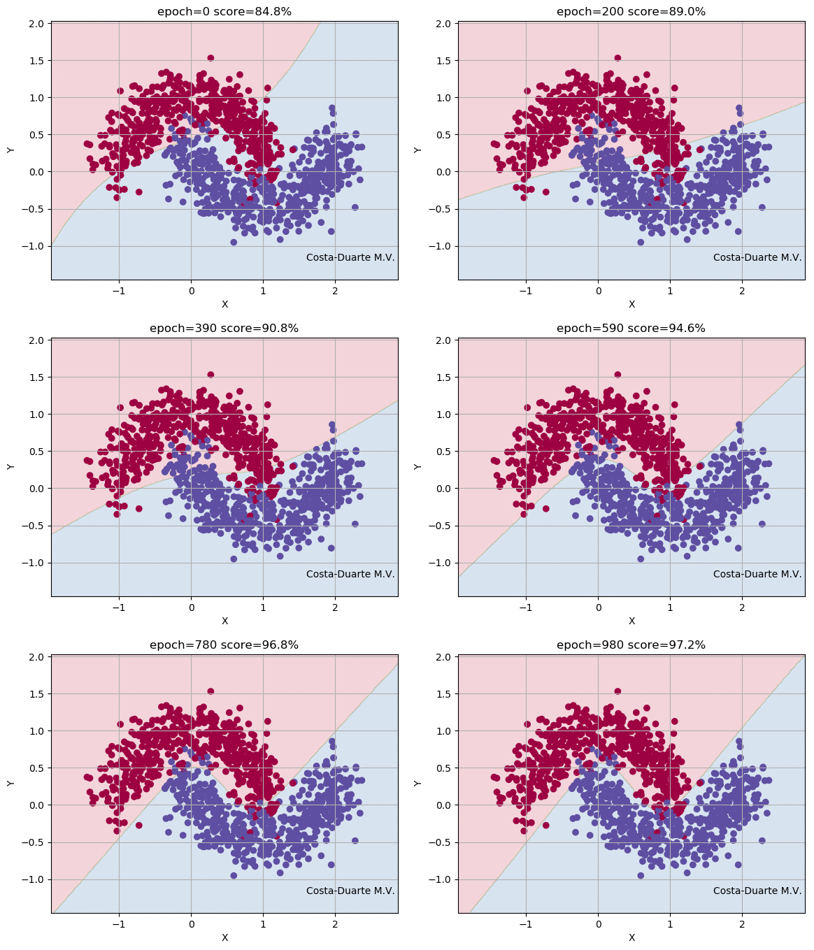
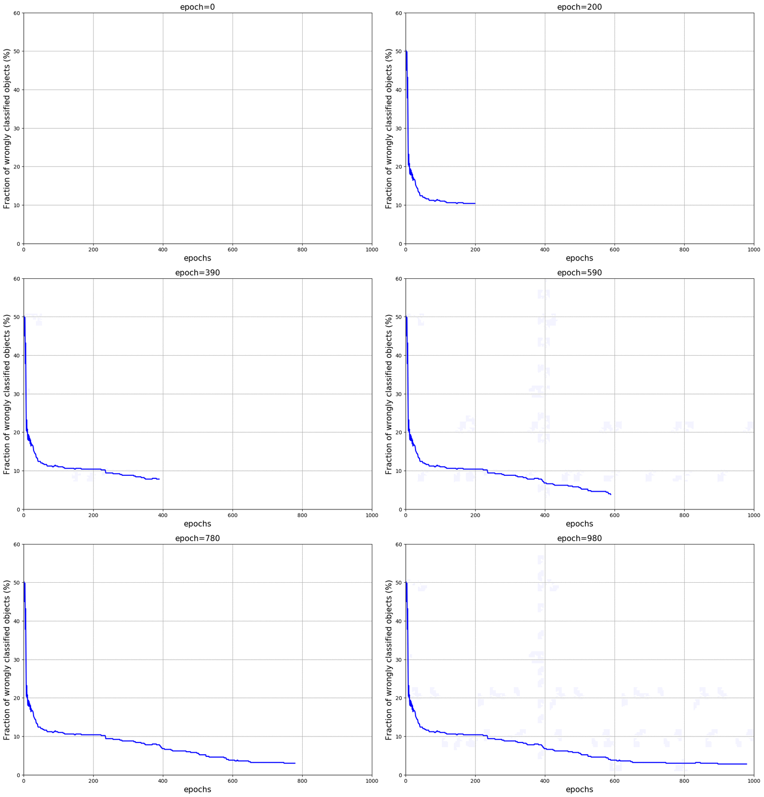
Using the dataset make_moons, we run our Neural Network over 1,000 iteractions, calculating the Foward and Back Propagations each epoch. Figure 2 shows the parameter space, some elements or objects of the training sample and the shaded area indicates the classification and its border between the two classes (red and blue). At the top of the animation, we can see the number of iteractions of the Neural Network and the score (fraction of objects in the training sample correctly classified). As the number of iteractions increases, the weights and bias terms get closer to the solutions and consequently the objects are correctly classified. The borders defined by the Neural Network between the groups becomes more efficient and well defined. Figure 3 shows the fraction of objects wrongly classified as a function of the iteraction. It is clear that the updated weights and bias arrays get closer to the minimal, providing high fraction of correctly classified elements in the validation sample. It is important to mention that the higher the number of nodes in the hidden layer or number of hidden layers, the better is the classification as the training runs. Again, the overfitting starts having an important role in this high-complexity models. The example shown in Figure 2 uses 10 nodes in the hidden layers and presented a score of 97% at the end of the iteractions. For this example, we used the sigmoid at the Input-Hidden Layers and the softmax at the Hidden-Output Layers. Of course you can play with that and change the activation functions (e.g. sigmoid(x) or ReLU(x)) showed before, but the equations derivated above slightly change.


Now you know how a Neural Network really works! If you are interested in playing a bit with this code, go to my Github and downloads the repository GitHub - Neural Network from Scratch. Remember to download the training/validation and test samples as well. Hereafter, you can also use other packages driven and optimized for Neural Network, such as Keras, Tensorflow and Theano. There are also other techniques to update weights and bias terms when your trainins sample is huge! Stochastic Gradient Descent and mini-batch Gradient Descent represent alternatives to train your Neural Network. If you have comments/suggestions about this post, please send me an e-mail.
Some references: