Marcus Duarte webpage

Artificial Neural Networks - Part 1: Foward Propagation

In this serie of Neural Network posts, I will demostrate how to implement the Artificial Neural Network (ANN) algorithm from scratch.

Nowadays, the expressions "Neural Network" and "Deep Learning" are quite fashion in the Big Data and Data Science tutorials and blogs. This algorithm was inspired by biological brain structures (neurons) and its complexity increased a lot since the 70s and 80s. Today, modern computers or clusters allow us to construct complex ANN to classify and predict values in diverse problems in many companies and Universities.

The ANN is composed by a collection of interconnected nodes (artificial neurons) distributed in layers. The connections are responsible to transmit the information from one neuron to another. Once the information arrives at a certain neuron or node, it is firstly processed and then transmited foward. Figure 1 shows the distribution of an ANN, composed by an Input Layer, one Hidden Layer (with $n_{hidden}$ nodes) and Output Layer. The arrows represent the connections between the nodes. In this context, the "Deep Learning" is commonly referred as a Neural Network with several hidden layers. Initially, the ANN is not able to properly to classify or predict anything. Since it is not trained, the weights and bias terms from all layers are not adjusted to carry out this task. To do so, we use namely two samples of data. The first one is the training sample, which is used to obviouly train the ANN and the second one is the test sample. The former one evaluates the performance of the trained algorithm after the training procedure. As a rule of thumb, the fraction between the training and test samples is around 70%/30% or 60%/40%. In this post, we explain the architecture of the ANN and how the training dataset passes through the Neural Network. The training procedure also needs the Back Propagation, which will be described in the next post.

**Figure 1**: The Artificial Neural Network composed by the Input Layer (2 nodes), the Hidden Layer (5 nodes) and Output Layer (2 nodes).

Mathematically, the ANN is a serie of matrix multiplication, including weights, input data and bias factors that enter at the left side and pass through the net up to the output layer at the right (Figure 1). Following the ANN showed above, the input and output layers contain 2 nodes. The training data is represented here by the matrix $X$ with dimensions ($n_{obj}, n_{feature})$. Between two consecutive layers, the data is multiplied by a weight factor and a bias factor is summed. It means that between the Input and Hidden Layers, we have the following matrix multiplication,

$$ z_1 = X * W_1 + b_1$$ being the dimensions of the weight and bias are equal to ($n_{feature}, n_{hidden})$ and ($n_{hidden}, 1)$, respectively. Note that the bias term $b_1$ is just an additive term and the dimension of $a_2$ is consequently ($n_{obj}, n_{hidden})$. The powerful skill of ANNs is represented by their capacity of complex and non-linearity modelling. Just considering the matrix multiplication above is not enough to reach such complexity. The next step is to pass our multiplication matrix result through an activation function, which decides whether it should be considered (or not) as a good or bad result for the layer, given the necessary complexity to fit the model to the data. There are many activation functions around but the main and most famous activation function is the sigmoid. Figure 2 shows the profile of the sigmoid(x) and others functions, such as tanh(x) and REctified Linear Unit aka ReLU(x).

**Figure 2**: The sigmoid(x), tanh(x) and ReLU(x) functions.

The values of the sigmoid function spam between 0 and 1 but it varies if one uses another activation function. The activated values of the Hidden Layer is then defined as $a_2 = g(z_1)$, where g is the activation function.

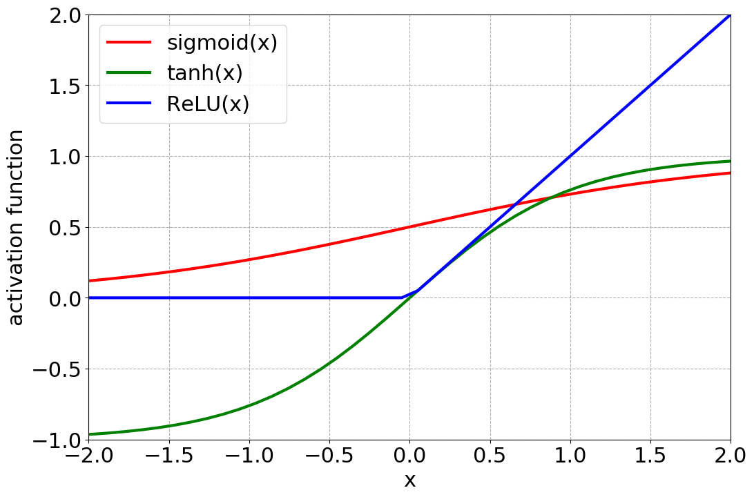
In the Python syntax, the activation function and the matrix multiplication between the Input and Hidden Layers can be written as,


              import numpy as np

defsigmoid(x): """ Sigmoid activation function """ if deriv == False: return 1.0 / (1.0 + np.exp(-x)) else: sigma = 1.0 / (1.0 + np.exp(-x)) return sigma * (1.0 - sigma) # Input -> Hidden Layer z1 = X.dot(W1) + b1 a2 = sigmoid(z1, deriv = False) Other activation functions in Python can be found in the link to my GitHub below.

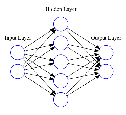
Similar procedure between the Input and Hidden Layers is done now between the Hidden Layer and the Output Layer. Note that now we use the output of the hidden layer $a_2$ as the new input. Thus,

$$a_3 = softmax(a_2 * W_2 + b_2)$$

Between the Hidden Layer and the Output Layer, we just use a different activation function. Here we use the softmax, which is a good choice for probability classifications. It can be written as, $$ softmax(x) = \frac{e^x}{\sum_i e^{x_i}}$$ In Python syntax, it is defined as the the softmax routine,

defsoftmax(x): """ Softmax activation function """ exp_x = np.exp(x) return exp_x / exp_x.sum(axis=1, keepdims=True) # Hidden -> Output Layer z2 = a2.dot(W2) + b2 a3 = softmax(z2)

Remember that the dimension of $a_2$ is ($n_{obj}, n_{hidden})$ and the weights and bias between the Hidden and Ouput Layers are represented as $W_2$ and $b_2$. For the matrix multiplication, their matricial dimensions are ($n_{hidden}, n_{output})$ and ($n_{output}, 1)$, respectively. The value $n_{output}$ represents the number of values atributed to each object in the Output Layer. This can be considered as classes or regression values. For instance, in case of bimodal classification, the output array length is 2 for each object in the training sample. In addition, it can be also considered as proabilities of this element to belong to classes, e.g., $[0.25, 0.75]$.

How many nodes should my ANN have? And how about the number of hidden layers? It really depends on how complex your data is. If you increase the number of nodes in the Hidden Layer, your model will be able to fit more complex and non-linear data. However, it will be more affected by overfitting, which is namely when your model only works on your training sample and fails on the test or any other sample. That's why it is so important to always evaluate the performance of your code with an independent (but representative) sample.

Increasing the number of hidden layers will consequently make your model more complex but you should think carefully before increasing the complexity of the ANN. Again, the overfitting can kill all your performance showing disapointing results on other samples. The increasing complexity also increases the computational time, particularly if your training sample is large enough. It can increase a lot your computational time, being most of time inpractical using an ordinary computer.

It is important to know how ANNs work but all this process above is already optimized by several packages in Python and R. Some examples are represented by Keras, Tensorflow and Theano. Some nice explanations of how ANN works are also in Data Science and Machine Learning blogs, then check the references below. If you want the full code of this post for didatic purposes, please check my GitHub - Neural Network from Scratch using the make_moons dataset. This post was just half of the story, the next part is the Neural Networks - Part 2: BackPropagation . If you have comments/suggestions about this post, please send me an e-mail.

Some references: